Coupled spring-mass system
| Date: | 2018-02-17 (last modified), 2009-01-21 (created) |
|---|
This cookbook example shows how to solve a system of differential equations. (Other examples include the Lotka-Volterra Tutorial, the Zombie Apocalypse and the KdV example.)
A Coupled Spring-Mass System
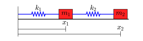
This figure shows the system to be modeled:

Two objects with masses $m_1$ and $m_2$ are coupled through springs with spring constants $k_1$ and $k_2$. The left end of the left spring is fixed. We assume that the lengths of the springs, when subjected to no external forces, are $L_1$ and $L_2$.
The masses are sliding on a surface that creates friction, so there are two friction coefficients, $b_1$ and $b_2$.
The differential equations for this system are
$m_1 x_1'' + b_1 x_1' + k_1 (x_1 - L_1) - k_2 (x_2 - x_1 - L_2) = 0$
$m_2 x_2'' + b_2 x_2' + k_2 (x_2 - x_1 - L_2) = 0$
This is a pair of coupled second order equations. To solve this system with one of the ODE solvers provided by SciPy, we must first convert this to a system of first order differential equations. We introduce two variables
$y_1 = x_1'$
$y_2 = x_2'$
These are the velocities of the masses.
With a little algebra, we can rewrite the two second order equations as the following system of four first order equations:
$x_1' = y_1$
$y_1' = (-b_1 y_1 - k_1 (x_1 - L_1) + k_2 (x_2 - x_1 - L_2))/m_1$
$x_2' = y_2$
$y_2' = (-b_2 y_2 - k_2 (x_2 - x_1 - L_2))/m_2$
These equations are now in a form that we can implement in Python.
The following code defines the "right hand side" of the system of equations (also known as a vector field). I have chosen to put the function that defines the vector field in its own module (i.e. in its own file), but this is not necessary. Note that the arguments of the function are configured to be used with the function odeint: the time t is the second argument.
def vectorfield(w, t, p):
    """
    Defines the differential equations for the coupled spring-mass system.

    Arguments:
        w :  vector of the state variables:
                  w = [x1,y1,x2,y2]
        t :  time
        p :  vector of the parameters:
                  p = [m1,m2,k1,k2,L1,L2,b1,b2]
    """
    x1, y1, x2, y2 = w
    m1, m2, k1, k2, L1, L2, b1, b2 = p

    # Create f = (x1',y1',x2',y2'):
    f = [y1,
         (-b1 * y1 - k1 * (x1 - L1) + k2 * (x2 - x1 - L2)) / m1,
         y2,
         (-b2 * y2 - k2 * (x2 - x1 - L2)) / m2]
    return f
Next, here is a script that uses odeint to solve the equations for a given set of parameter values, initial conditions, and time interval. The script writes the points to the file 'two_springs.dat'.
# Use ODEINT to solve the differential equations defined by the vector field
from scipy.integrate import odeint

# Parameter values
# Masses:
m1 = 1.0
m2 = 1.5
# Spring constants
k1 = 8.0
k2 = 40.0
# Natural lengths
L1 = 0.5
L2 = 1.0
# Friction coefficients
b1 = 0.8
b2 = 0.5

# Initial conditions
# x1 and x2 are the initial displacements; y1 and y2 are the initial velocities
x1 = 0.5
y1 = 0.0
x2 = 2.25
y2 = 0.0

# ODE solver parameters
abserr = 1.0e-8
relerr = 1.0e-6
stoptime = 10.0
numpoints = 250

# Create the time samples for the output of the ODE solver.
# I use a large number of points, only because I want to make
# a plot of the solution that looks nice.
t = [stoptime * float(i) / (numpoints - 1) for i in range(numpoints)]

# Pack up the parameters and initial conditions:
p = [m1, m2, k1, k2, L1, L2, b1, b2]
w0 = [x1, y1, x2, y2]

# Call the ODE solver.
wsol = odeint(vectorfield, w0, t, args=(p,),
              atol=abserr, rtol=relerr)

with open('two_springs.dat', 'w') as f:
    # Print & save the solution.
    for t1, w1 in zip(t, wsol):
        print >> f, t1, w1[0], w1[1], w1[2], w1[3]
The following script uses Matplotlib to plot the solution generated by the above script.
# Plot the solution that was generated

from numpy import loadtxt
from pylab import figure, plot, xlabel, grid, hold, legend, title, savefig
from matplotlib.font_manager import FontProperties

t, x1, xy, x2, y2 = loadtxt('two_springs.dat', unpack=True)

figure(1, figsize=(6, 4.5))

xlabel('t')
grid(True)
hold(True)
lw = 1

plot(t, x1, 'b', linewidth=lw)
plot(t, x2, 'g', linewidth=lw)

legend((r'$x_1$', r'$x_2$'), prop=FontProperties(size=16))
title('Mass Displacements for the\nCoupled Spring-Mass System')
savefig('two_springs.png', dpi=100)

Section author: WarrenWeckesser, Warren Weckesser
Attachments